subunit2sql-graph
subunit2sql includes a utility to generate various graphs from the data in a database. This is used to provide a more visual analysis of the data contained in the DB.
Installing subunit2sql-graph
The subunit2sql-graph entry point will be installed when you run install on the subunit2sql endpoint. However, there are a couple of additional dependencies needed to use it. These are listed as setuptools extras as they are fairly heavyweight and depend on several C libraries being present. To install the additional dependencies to use the graph command you can use:
pip install subunit2sql[graph]
or:
pip install $PATH_TO_subuni2sql[graph]
For example:
git clone https://git.openstack.org/openstack-infra/subunit2sql .
pip install -e .[graph]
Using subunit2sql-graph
After you install subunit2sql and the additional dependencies you invoke the graph command with:
subunit2sql-graph
It is required that you also specify a database to tell the graph command to tell the graph command how to connect to the DB to use for generating the graph. This is done using the same syntax as other subunit2sql commands:
subunit2sql-graph --database-connection mysql://subunit:pass@127.0.0.1/subunit
The other common required argument is the output file which is -o or –output. This arg is a straight passthrough to a matplotlib call which uses the extension to generate the graph file. So make sure you’re using the file format extension you want the output to be generated in.
You then provide a graph subcommand to tell subunit2sql-graph which type of graph to generate and provide any args needed to the command. Also, note that graph specific args must come after the graph on the CLI and general args must come before. This will likely change in the future, but at least for right now it’s an existing issue.
There are currently 4 graphs that it can generate:
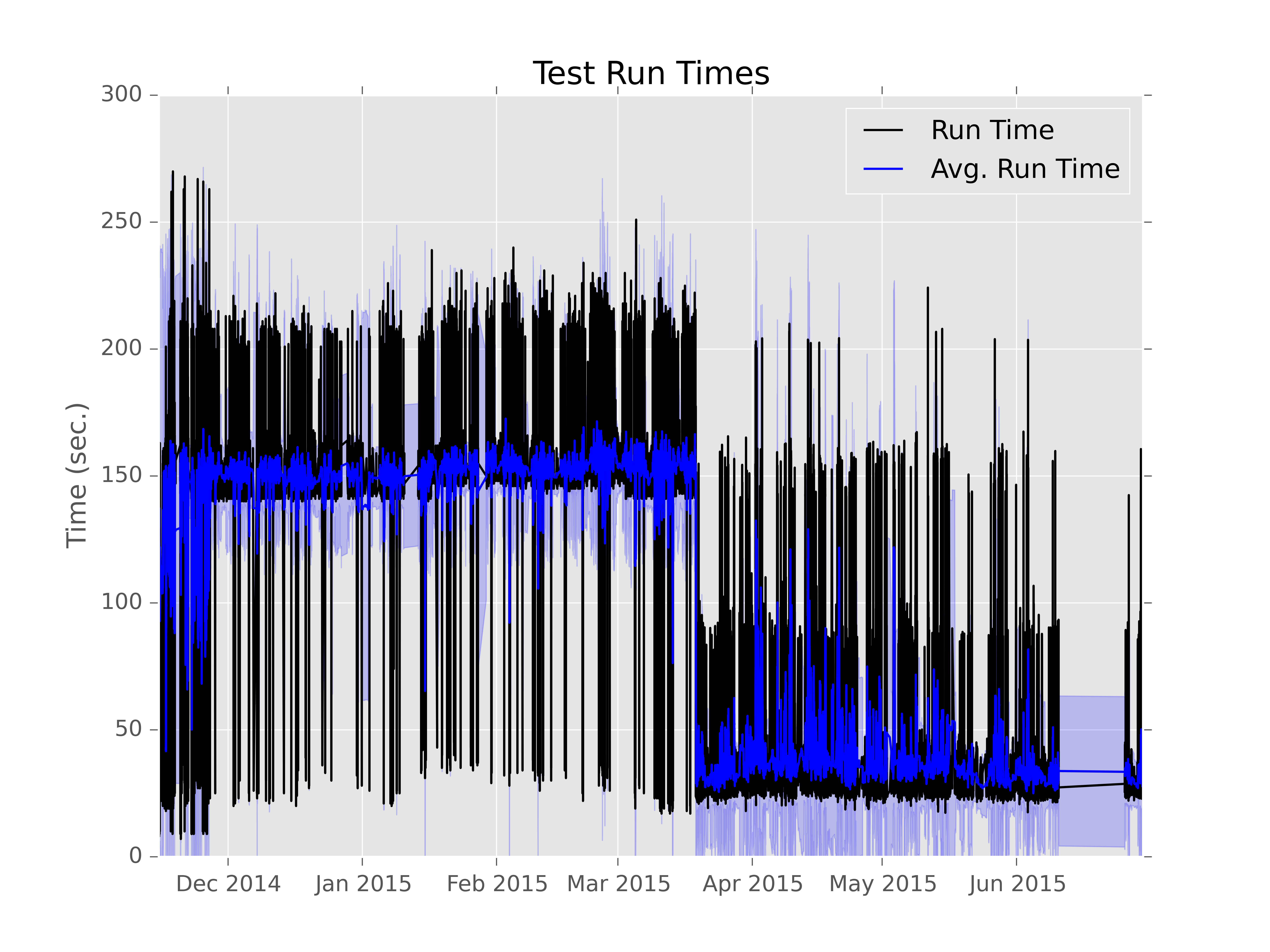
Run Time
This graph is used to show the run time of a single test over time. It generates a line graph displaying the time series data for successful run times for the specified test from the test_runs table.
For example running something like:
subunit2sql-graph --database-connection mysql://test:test@localhost/subunit2sql --output test.png --title 'Test Run Times' run_time tempest.api.identity.admin.v2.test_users.UsersTestJSON.test_update_user_password
will generate a graph like:
you can refer to the help on the graph command for run_time to see the full option list with something like:
subunit2sql-graph run_time --help
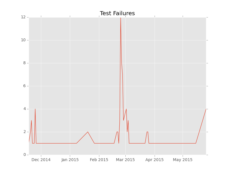
Failures
This graph is used to show the number of failures, successes, and skips of a single test over time. It generates a line graph displaying the time series data for each of these counts (grouped daily) as different line plots on the same graph.
For example running something like:
subunit2sql-graph --database-connection mysql://test:test@localhost/subunit2sql --output test.png --title 'Test Failure Count' failures tempest.api.compute.servers.test_server_actions.ServerActionsTestJSON.test_rebuild_server
will generate a graph like:
The command will also display the percentages of each status category, for example with the above command something like:
Fail Percentage: 0.2045%
Success Percentage: 99.7955%
Skip Percentage: 0.0000
will be printed to STDOUT.
You can refer to the help on the graph command for run_time to see the full option list with something like:
subunit2sql-graph failures --help
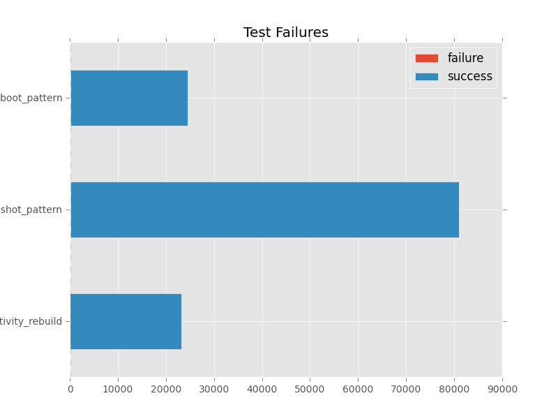
Aggregate Counts
This graph is used to show the aggregate number of failures, successes, and skips of multiple tests from the database. It a stacked bar graph showing the count of each category for all the provided tests. If no tests are provided this graph tries to use all the tests from the DB. (which depending on the data set can be difficult to render)
For example running something like:
subunit2sql-graph --database-connection mysql://test:test@localhost/subunit2sql --output test.png --title 'Test Failure Failures' agg_count
will generate a graph like:
you can refer to the help on the graph command for run_time to see the full option list with something like:
subunit2sql-graph failures --help
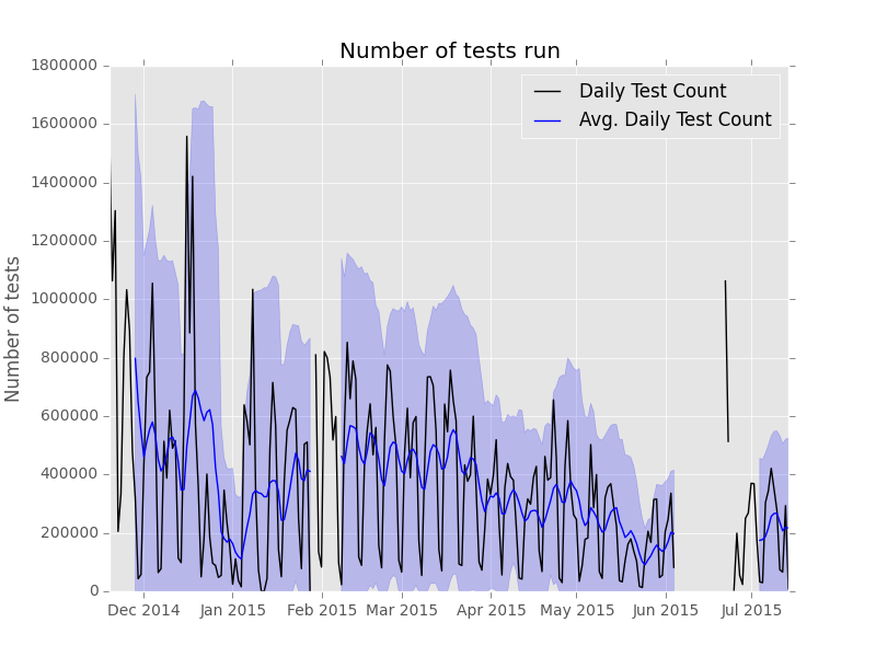
Daily Test Counts
This graph is used to show the the daily # of tests run as a time series line graph.
For example, running something like:
subunit2sql-graph --database-connection mysql://test:test@localhost/subunit2sql --output test.png --title 'Daily Test Count' dailycount
will generate a graph like:
Run Time Grouped By Run Metadata
This graph generates a box and whiskers plot to show the distribution of run times for runs with each plot grouped by values to a provided run_metadata key
For example, running something like:
subunit2sql-graph --title "Run times by Job Name" --database-connection mysql://test:test@localhost/subunit2sql -o test.png run_time_meta build_name --filter_list gate-tempest-dsvm-neutron-full-ssh,gate-tempest-dsvm-full-ubuntu-xenial,gate-tempest-dsvm-full-ubuntu-trusty,gate-tempest-dsvm-py35-ubuntu-xenial
will generate a graph like:
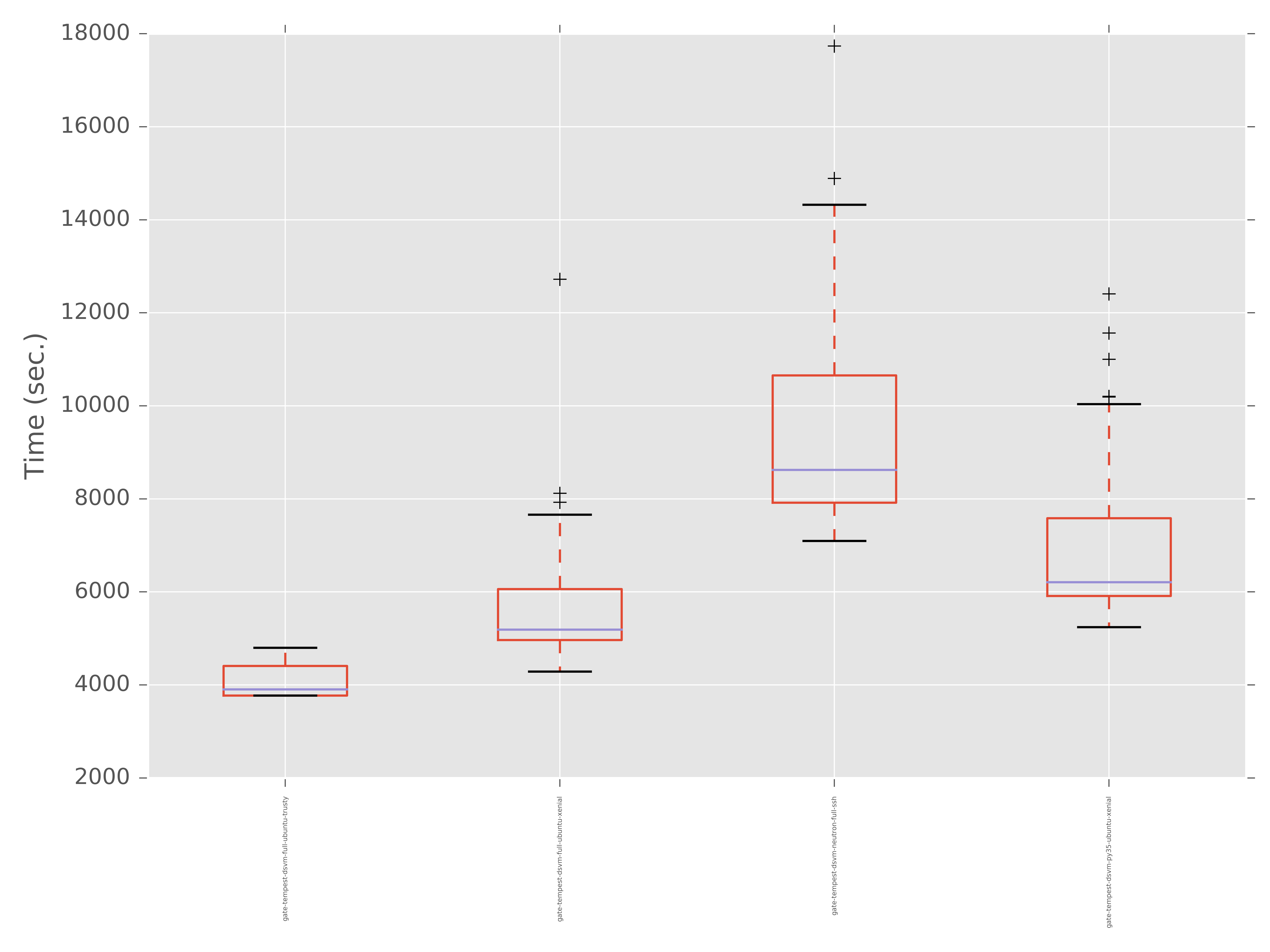
It’s also worth noting the –filter_list argument used in the command above. In some cases, especially larger data sets, there are too many distinct values for a given run_metadata key to make the graph useful. To workaround this you specify a list of values that will be used to filter the output so that only matches of that key will be in the output.
Run Failure Rate Grouped By Run Metadata
This graph generates a bar chart to show the failure rates for all runs for with a run_metadata value for a user provided run_metadata key.
For example, running something like:
subunit2sql-graph --title "Failure Ratess by Job Name" --database-connection mysqll://test:test@localhost/subunit2sql -o test.png run_failure_rate build_name --filter_list gate-tempest-dsvm-neutron-full-ssh,gate-tempest-dsvm-full-ubuntu-xenial,gate-tempest-dsvm-full-ubuntu-trusty,gate-tempest-dsvm-py35-ubuntu-xenial
will generate a graph like:
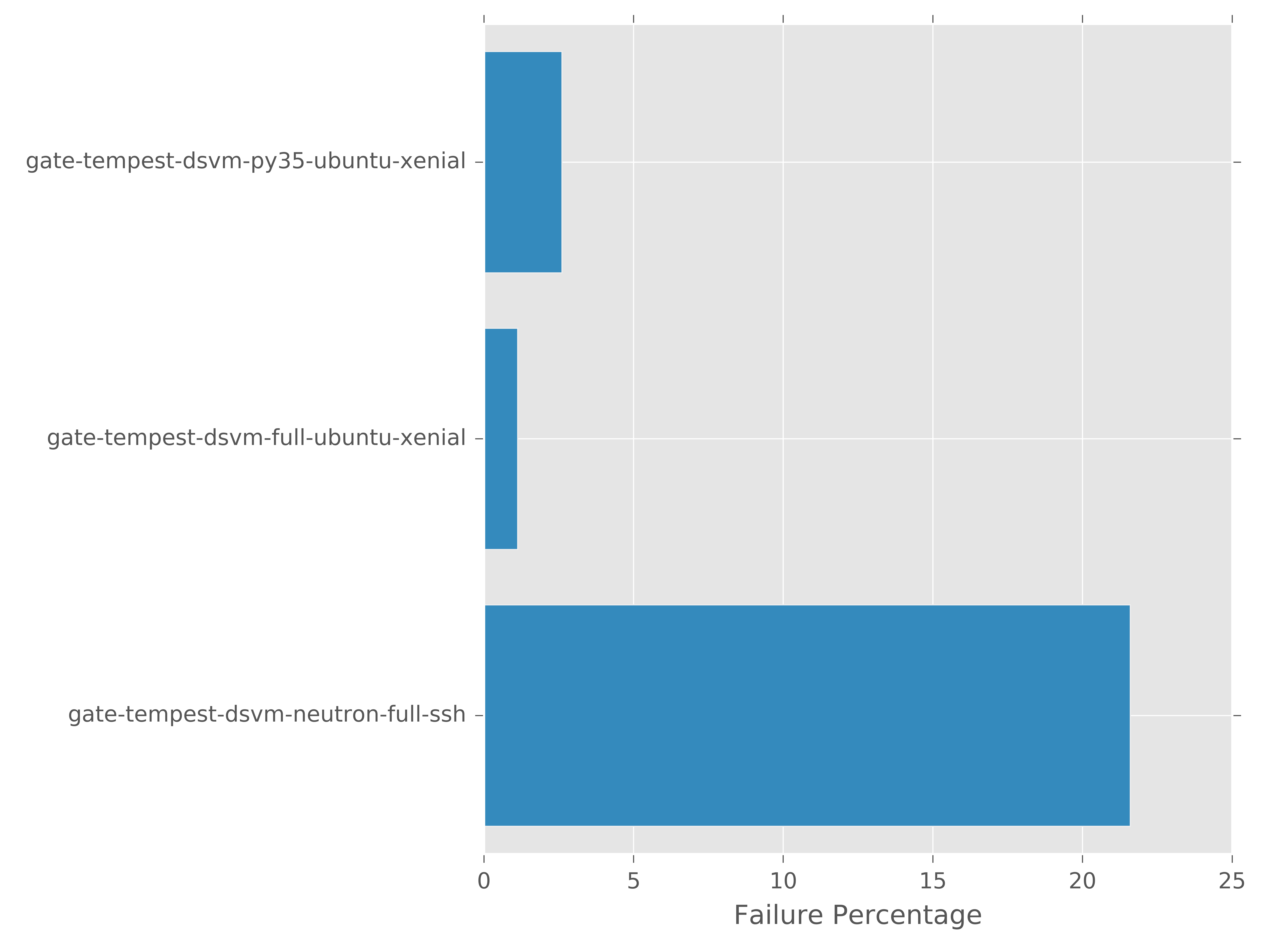
It’s also worth noting the –filter_list argument used in the command above. In some cases, especially larger data sets, there are too many distinct values for a given run_metadata key to make the graph useful. To workaround this you specify a list of values that will be used to filter the output so that only matches of that key will be in the output.
subunit2sql-graph plugin interface
subunit2sql-graph exposes a plugin interface which enables others to add additional graph types to the command without having to add the additional modules to the subunit2sql repository. This could be because the additional graph commands are too application specific to be in the general purpose command, or really any reason.
A graph plugin is simply a python module that has of a few pieces: a set_cli_opts function, a generate_series function, and a python entrypoint. This is the same as the internal interface for the in-tree commands, meaning that migrating a command from landing in the upstream repo and as an external plugin is quite straightforward.
Entry Point
This is how you tell the subunit2sql-graph command about the existence of the external plugin. It leverages setuptools and stevedore to register the module in a known namespace which will be loaded by the subunit2sql-graph command.
To add a plugin you just need to add an entry-point for your new graph command to the ‘subunit2sql.graph.plugin’ namespace. For example, if you were adding a plugin for the new command graph_pretty_results you would use the following in your setup.cfg (assuming you’re using PBR):
[entry_points]
subunit2sql.graph.plugin =
    graph_pretty_results = path.to.plugin.module
Then after you install the python program the plugin is in the subunit2sql-graph will be able to use the plugin.
The plugin module
There are a couple of requirements for each plugin module. First you’ll need to import oslo.config and setup a CONF object. This can be done very simply with:
from oslo_config import cfg

CONF = cfg.CONF
This is needed so you’ll be able to parse some required CLI opts from the base command like the output directory.
Additionally, there are some required functions in the plugin which are described in the sections below.
For examples, of how to write a plugin module you can look at any of the in-tree graph commands they are constructed in the same exact way as an out-of-tree plugin.
set_cli_opts function
This function is used to set any command specific options. It takes in a single parameter a ConfigParser object which is used to register options on. The function is required even if no additional command specific options are needed. Simply add it and make it a no-op, for example:
def set_cli_opts(parser):
    pass
The normal way this is used is to add args is to just call add_argument on the parser passed in. For example, to add a single option, test_id, you would do the following:
def set_cli_opts(parser):
    parser.add_argument('test_id', nargs='?',
                        help='Test id to extract time series for')
generate_series function
This is where all the actual work for generating the graph in the plugin happens this function is where the graph is generated and the output is saved to a file. Basically when you run subunit2sql-graph with your plugin as the graph type this is the function which gets called to do the work.
There are a couple of constraints in how it functions. First, the use of the oslo_config config object is how to get at CLI arg values. Base command values are in the default namespace, for example CONF.output. You can see the list of available options from the SHELL_OPTS list in subunit2sql/analysis/graph.py Command specific options are available in the command namespace. For example, if you add set an arg “test_id” in set_cli_opts() then you can get to the value of it from CONF.command.test_id.
The other constraint on this function is that the way it gets called by subunit2sql-graph assumes that it will be writing an image file. The last thing subunit2sql-graph does is print “Graph saved at: file_path” The file_path is whatever CONF.output is set to so you should use that for the output path. The other aspect is the file extension of this value is used to specify the file format of the image file. The file output commands from matplotlib, which is what is used for all the in-tree commands, will take care of this automatically. However using matplotlib is not a requirement, just make sure however you generate a graph respects the file extension of the output path.
